
Do you realize how risky it can be for a company’s data to contain repeated values (duplicates)? Yes! The data tends to be difficult to interpret as a result of these duplicate values. Duplicates ultimately overestimate your results, too. Good news! One can use Excel to eliminate duplicate files from business‘s data. Similarly, do you have a lengthy list of data on Excel and are searching for a specific one with the data recorded regarding it? Not to worry! On this page, you will discover a straightforward technique that will quickly deliver the information you seek. Yes! It is known as XLOOKUP.
On this topic of how to remove duplicates and use XLOOKUP in Excel, let’s start by discussing how to remove duplicates in Excel. For better comprehension, I’ll also include an illustration.
Table of Contents
How To Remove Duplicates in Excel
Step 1: Select the data that you want to search for the duplicates
To delete a group of cells with duplicate values, right-click down that group of cells (check image 1)

Image 1: Selected Data
For instance, I want to get rid of names, user IDs, and usernames that appeared multiple times. The 25 rows and the three columns (A, B, and C) are highlighted.
Step 2: Look for the Data button in the Menu bar after selecting the cell range
A drop-down menu will appear if you right-click on it (see image 2). Now! Scroll to Remove Duplicates.

Image 2 – Drop Down to Remove Duplicates
Step 3: Select Remove duplicates with a right-click
A page containing details on the column for which you want to fix the duplicate issue will appear.
Please, be aware that the Remove Duplicate page will only display the numbers of the columns you have highlighted. Select Remove Duplicates after checking the relevant boxes.

Image 3 – Remove Duplicates Page
I want to remove the duplicates in columns A, B, and C, for instance. As a result, I highlighted the columns to be treated. You’ll realise that the only visible columns on this page are the ones I highlighted.
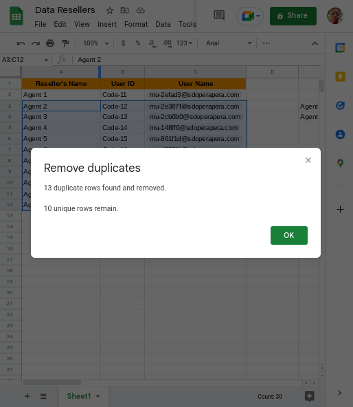
Image 4 – Data without Duplicates
If, however, at this point, you change your mind and decide to omit a column, check that box and continue. Yes! Now try one yourself.
How to Remove Duplicates in Excel Without Changing the Data Sequence
Do you want to remove the duplicate item from your file without tampering with the arrangement?
Most businesses would object to tampering with the order of their data. Here is another method for simply removing duplicates from your data. However, this method has a formula that you need to cram.
=COUNTIF($A$2:$A2,$A2)>1
The formula will make it easier for you to spot the duplicates. You just need to get the actual application of this formula after I show you how to use it.
Step 1: Highlight the data to be checked for duplication (check image 1 to do this).
Step 2: Select the Format option from the Menu bar. Right-click on Conditional formatting at the bottom of the drop-down. You will see image 5.

Image 5 – Conditional Formatting
Step 3: Click on format cells if… under the format rules to bring up a drop-down menu. Input the following formula in the next tab below by clicking the Custom Formula is… button: =COUNTIF($A$2:$A2,$A2)>1.

Image 6 – Conditional Format rules
You can adjust the colour to your preference. Click Done once you’ve completed this.

Image 7 – Duplicate value in Yellow
The duplicate data will automatically be highlighted, and you can now manually remove them.
Having analyzed how to remove duplicates from your business’ data, let’s move on to how to use Xlookup in Excel.
How to Use XLOOKUP in Excel
XLOOKUP is a recently developed function that searches a table for data. The XLOOKUP function looks for the first match within a range and then returns the information corresponding to that match. However, XLOOKUP will return the closest match if there isn’t one.
As an illustration, you can use XLOOKUP to look up an employee’s information using their ID.
Excel’s XLOOKUP feature was first added as a beta function in August 2019, and now it’s only accessible through Microsoft 365. (July 2021).
After describing what XLOOPUP is all about, let’s move on to how to use XLOOKUP to verify data in four simple steps.
Step 1: First, you need to choose a cell and type =XLOOKUP.
Step 2: Next, select the element you want to evaluate. Then, you should insert the lookup value into a different cell. Once you’ve done that, type a comma.
Step 3: After selecting the cells you want to search for the value in, add a comma. Now choose the cells that contain the information you wish to return.
Step 4: Enter the information you need by pressing the Enter key on your keyboard.
Final Thoughts on How To Remove Duplicates and Use XLOOKUP in Excel
We have discussed how to remove duplicates and use XLOOKUP in Excel in this article. Additionally, we discussed how to spot duplicates in the colour of your choice.
Additionally, you’ve mastered using Xlookup to conduct detailed searches across a long list of data.